How UAV Teams Cut Prototype Iterations by 40% — With the Right Simulation Setup

The Problem No One Talks About

You tuned the geometry for three weeks. The prototype flew — but endurance was 18% below predicted, and motor mounts were running 24°C hotter than your thermal model showed.

This is not a hardware failure. It is a simulation setup failure.

The gap between simulation output and real-world UAV performance almost always traces back to three things:

• Wrong turbulence model for low Reynolds number rotary flow
• Underdefined thermal boundary conditions
• Insufficient mesh density around blade tip vortex regions

This guide breaks down how to fix all three — using Ansys Fluent, Ansys Mechanical, and Ansys Icepak in a coupled multiphysics workflow.

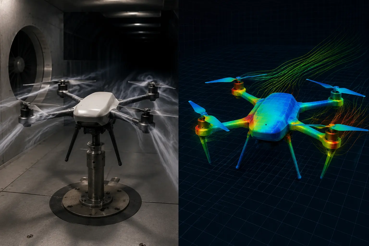
Why UAV Aerodynamics Is Harder to Simulate Than Most Engineers Expect

UAVs operate in a regime where standard simulation assumptions break down — Re 50,000–500,000, where flow is neither cleanly laminar nor fully turbulent.

The four specific failure points:

1. 1
   Laminar Separation Bubbles at Low ReAt Re < 200,000, boundary layers separate before transitioning back to turbulent flow. Standard k-ε models miss this entirely. The result: lift coefficient predictions off by 15–25%.
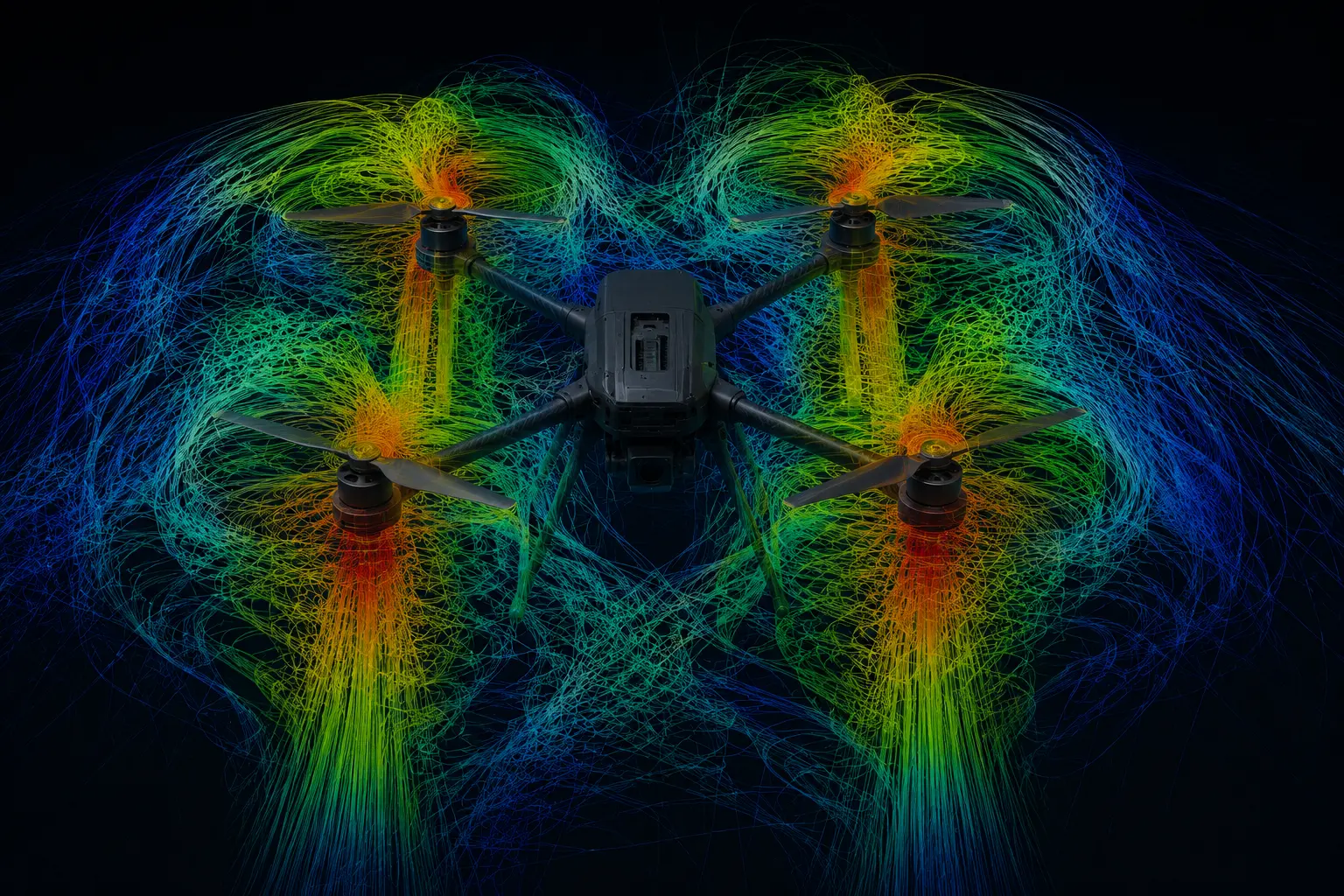
2. 2
   Rotor-Rotor Interference in Multi-Rotor SystemsSimulating one rotor and multiplying by four introduces systematic error. Wake interference between rotors reduces effective thrust by 8–14% — and this shows up directly in your flight endurance predictions.
3. 3
   Fluid-Structure Interaction on Carbon Fiber BladesA 12-inch CFRP prop at cruise conditions can see 3–8mm tip deflection. That changes effective pitch, which changes thrust and efficiency. Pure CFD without structural coupling gives you optimistic numbers.
4. 4
   MRF vs Sliding Mesh — Choosing Wrong Costs You AccuracyMRF is adequate for hover. In forward flight, it introduces 12–18% thrust prediction error because rotor-body interaction is periodic, not steady.

Turbulence Model Selection — The Decision Most Engineers Get Wrong

Fixed-wing UAVs and blades (Re 50,000–500,000)

Use Gamma-ReTheta Transition SST in Ansys Fluent. It captures laminar-to-turbulent transition — specifically the separation bubble behaviour that two-equation models cannot model. Do not use Realizable k-ε here. It will predict attached flow where the flow is actually separating and reattaching.

For blade angles of attack above 10–12°, use Detached Eddy Simulation (DES) in Ansys Fluent 2023 R1+. Compute cost is ~3× RANS, but accuracy on separated flow cases justifies it.

Hover analysis — high-Re rotors (Re > 500,000)

Realizable k-ε with enhanced wall treatment is sufficient for macro thrust and torque predictions (within 5–8% of experimental). Use MRF for design iteration, switch to Sliding Mesh for final validation and any forward flight case.

Full UAV body — external aerodynamics in forward flight

SST k-ω is the recommended baseline. Enable curvature correction — a single checkbox in Fluent — to account for streamline curvature in propeller wake regions.

Topology Optimisation — Build Less, Hold More

Most UAV frames are overbuilt in the wrong places. Topology optimisation in Ansys Mechanical finds where your structure is carrying load — and where it isn't — before you cut a single piece of material.

The process is straightforward: define your design space, apply real-world load cases (max thrust, gust loads, motor torque, landing impact), set what geometry must stay fixed (motor mounts, battery bay, fastener zones), and let the solver find the most efficient load path.

What actually matters in the setup

Run it across all flight load cases — not just hover. A frame optimised for hover alone will be fragile in forward flight and on landing. Set your retained mass target at 30–50% of the original design space. Go below 30% and the output becomes difficult to manufacture or validate.

What to expect

Typically 25–40% weight reduction while retaining 90–95% of original stiffness. One important note: the output is a density map, not a finished geometry. You remodel the optimised shape in CAD, then re-run a full stress check on the final design. It's a direction, not a destination.

The teams that get the most value from this run it early — before tooling decisions, not after.

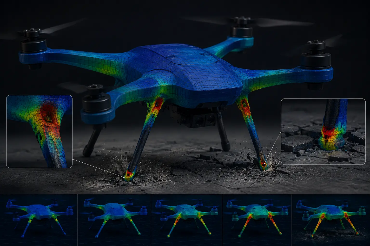
Drop Test Simulation — Know If Your Landing Gear Survives Before It Has To

A failed landing gear on a 5kg UAV at 2.5 m/s costs you a prototype, a battery pack, and weeks of redesign. This is one of the most avoidable failures in UAV development — because it's entirely simulatable before the first unit is built.

What to simulate

A vertical descent at 2–3 m/s at maximum take-off weight. This covers a firm landing or a low-altitude power-loss event — the two most common structural failure scenarios in field operations. For UAVs above 10kg MTOW, add a 4 m/s case as well.

The right solver

Use Explicit Dynamics in Ansys Mechanical. Standard structural solvers aren't built for impact — contact forces change too fast. Explicit dynamics captures the full event in milliseconds, including peak stress, deformation, and energy absorption, accurately.

Three numbers to focus on after the run

• Peak stress at the leg root — compare this against your material's proof stress. If it exceeds it, the leg will bend permanently on the first hard landing.
• Energy split — your landing gear should absorb more than 60% of the impact energy. If the airframe is taking more than 40%, the design is transferring the problem upstream.
• Permanent deformation — if the leg spread increases by more than 5mm after a single impact, it won't survive repeated use in the field.

The simulation takes a fraction of the time and cost of a physical drop test. More importantly, it gives you the data to make a design decision — not just observe a failure.

Mesh Setup — Where Inaccurate Results Actually Start

Blade and propeller meshing

• Target y+ ≤ 1 for Transition SST (wall-resolved). For k-ε with wall functions, y+ 30–300 is acceptable — verify post-solve via Fluent wall y+ contour plots
• Smallest cell at blade tip ≤ 2% of local chord length
• Minimum 15 inflation layers. First layer height sized to target y+. Growth ratio: 1.2

Domain sizing

• Forward flight: 10 body lengths upstream, 20 downstream, 10 lateral
• Hover: cylindrical domain preferred — radius ≥ 8× rotor diameter, 5× above and 10× below

Cell count benchmarks

• Isolated propeller hover (RANS, MRF): 2–5 million cells minimum
• Full quadcopter hover (4 rotors + frame): 15–40 million cells
• Fixed-wing in forward flight (SST k-ω): 8–20 million cells

Below these numbers, your results are numerically diffused — not converged.

Polyhedral vs tetrahedral

Polyhedral meshing in Fluent requires 50–70% fewer cells for equivalent accuracy and converges 30–40% faster. This directly reduces HPC compute cost per run.

Structural Analysis — What to Run and in What Order

Start with modal analysis — always

Calculate blade passing frequency: RPM ÷ 60 × number of blades.

Example: 2-blade 10-inch props at 8,500 RPM → 283 Hz blade passing frequency.

Extract the first 20 natural frequencies of your assembled frame in Ansys Mechanical. Any structural mode within ±15% of the blade passing frequency or its harmonics is a resonance risk. This is the cheapest simulation you will run — and the most consequential.

Fatigue life analysis

• Input: variable amplitude load history from your flight profile (CFD pressure export or measured flight data)
• Output: fatigue damage factor contour across the structure — zones approaching 1.0 are predicted failure locations
• For CFRP structures: use Ansys Composite PrepPost (ACP) for ply-by-ply stress analysis — failure in composites is direction-dependent

Landing impact

Simulate a 2–3 m/s vertical descent at MTOW using explicit dynamics in Ansys Mechanical. Evaluate peak stress, deformation, and energy absorption before committing to a landing gear design.

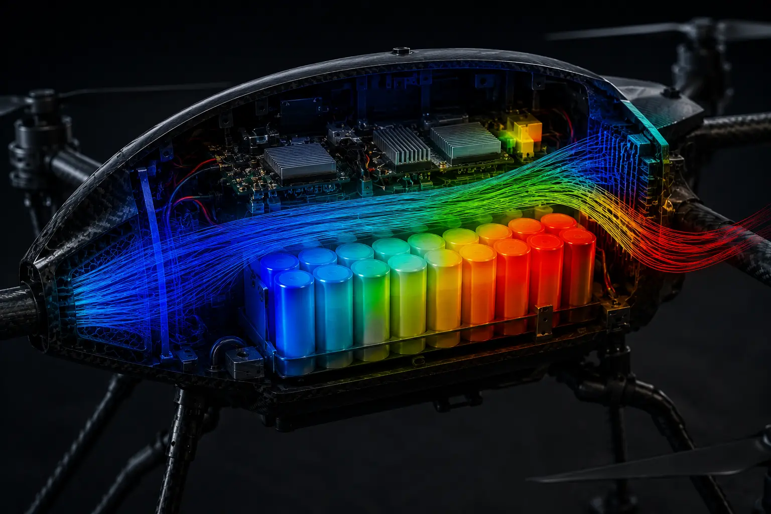
Battery and Electronics Thermal — Simulate Before You Seal the Airframe

Battery packs above 45°C degrade faster. Above 60°C, thermal runaway risk becomes real. If you are validating thermal management after the prototype is assembled, you are already late.

Battery thermal setup in Ansys Icepak

Model each cell as a volumetric heat source. Heat per cell = I² × R_internal (use temperature-dependent values from the manufacturer datasheet).

Example calculation — 4S 5000mAh LiPo at 20C discharge (100A)

• R_internal per cell: 3–5 mΩ
• Heat per cell: ~4–8W
• 4S pack with 2P configuration = 8 cells → 32–48W total pack heat load

Run conjugate heat transfer (CHT) to model airflow through the airframe. Target output: steady-state temperature across each cell, ESC, and motor controller. Flag any hotspot exceeding 45°C (Li-ion) or 55°C (LiPo) under worst-case discharge.

Coupling aerodynamics with thermal

In Ansys Workbench, link Fluent external aero output directly to Icepak as inlet boundary conditions. This replaces assumed uniform airflow with actual velocity and turbulence intensity data — significantly more accurate for enclosure thermal predictions.